Quality control of metapreotomics data

Set-up environment

## libraries
library(tidyverse)


# input data

# Metaproteomics quality control data from MaxQuant
df_qc <- read.table("../../project/rawdata/final_summary.tsv",
                    header = TRUE,
                    sep = "\t",
                    check.names = FALSE)
# Metadata
metadata <- read.table("../../project/rawdata/metadata_metapro.txt",
                       header = TRUE,
                       sep = "\t"
                       )

Clean metadata

metadata_clean <- metadata %>%
  rename(sample = Probenname) %>%
  mutate(sample = str_replace_all(sample, "\\.", "_")) %>%
  separate(Abschnitt,
    into = c("region", "source",
      sep = " "
    )
  )

Clean quality data

clean_qc <- df_qc %>%
  select(
    "Raw file",
    "Peptide Sequences Identified",
    "MS/MS Identified",
    "MS/MS Identified [%]"
  ) %>%
  rename(
    sample = "Raw file",
    peptide_identified = "Peptide Sequences Identified",
    ms_identified = "MS/MS Identified",
    ms_identified_perc = "MS/MS Identified [%]"
  ) %>%
  filter(sample != "Total")

Create a summary table

max(clean_qc$peptide_identified)

[1] 27841

sapply(clean_qc[2:4], mean)

peptide_identified      ms_identified ms_identified_perc 
         10646.400          17453.600             26.159

summary_table <- data.frame(
  stats = c("Max", "Mean", "Min"),
  peptide_identified = round(c(25687.0, 11420.1500, 472.00)),
  ms_identified = round(c(28442.0, 13235.5000, 766.00)),
  ms_identified_perc = round(c(29.9, 14.8755, 0.98), 2)
)

summary_table

  stats peptide_identified ms_identified ms_identified_perc
1   Max              25687         28442              29.90
2  Mean              11420         13236              14.88
3   Min                472           766               0.98

write.csv(summary_table, "../../project/rawdata/summary.csv")

Pivot data

pivoted_data <- clean_qc %>%
  pivot_longer(-(sample), names_to = "qc", values_to = "value")

head(pivoted_data)

# A tibble: 6 × 3
  sample qc                    value
  <chr>  <chr>                 <dbl>
1 10_1   peptide_identified   642   
2 10_1   ms_identified       1045   
3 10_1   ms_identified_perc     1.96
4 10_18  peptide_identified 24411   
5 10_18  ms_identified      36628   
6 10_18  ms_identified_perc    54.6

Plot the data

 pivoted_data %>%
  filter(qc=="peptide_identified") %>% 
   ggplot(aes(x=value,
             y=sample)) +
  geom_bar(stat = "identity") +
  geom_vline(aes(xintercept=mean(value)),
              color="blue", linetype="dashed") +
  scale_x_continuous(expand = c(0,0),
                     limits = c(0, 29000),
                     breaks=seq(0, 29000, by=3000)) +
  labs(x="",
       y="Number of identified peptides") +
  theme_classic()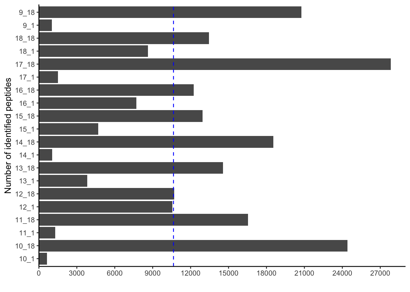

 pivoted_data %>%
   filter(qc=="peptide_identified") %>%
  ggplot(aes(x=sample,
             y=value)) +
  geom_point(size=4)+
  geom_hline(aes(yintercept=mean(value)),
             color="blue", linetype="dashed") +
  scale_y_continuous(expand = c(0,0),
                     limits = c(0, 27000),
                     breaks=seq(0, 27000, by=3000)) +
  labs(x="",
       y="Number of identified peptides") +
  theme_classic()

Warning: Removed 1 rows containing missing values (`geom_point()`).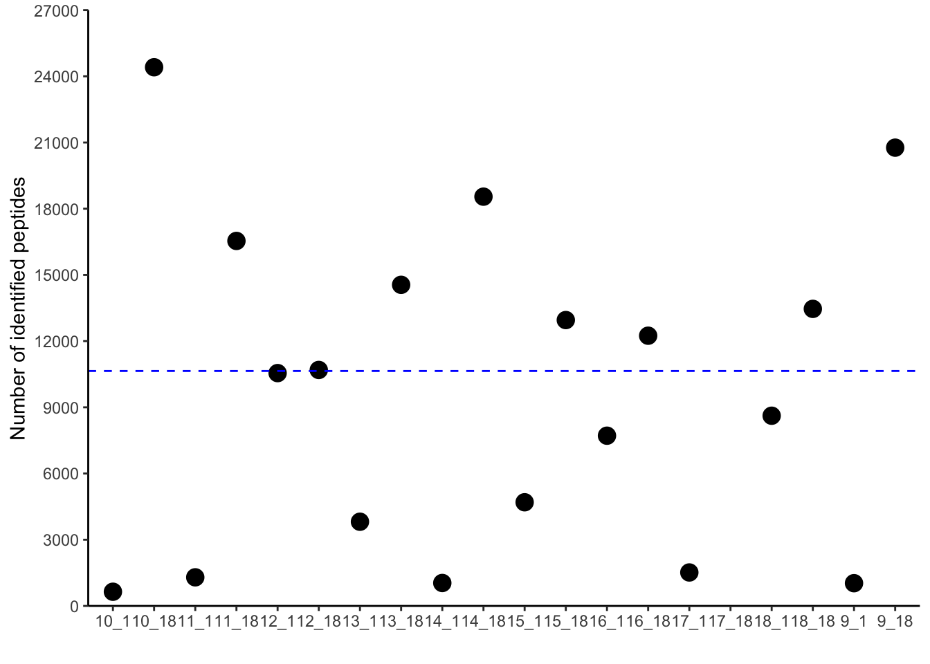

 pivoted_data %>%
  filter(qc=="peptide_identified") %>%
  ggplot(aes(x="peptides",
             y=value)) +
  geom_boxplot(width = 0.3)+ 
  geom_jitter(width = 0.1,
              size = 3,
              color = "red",
              alpha = 0.6) +
  scale_y_continuous(expand = c(0,0),
                     limits = c(0, 29000),
                     breaks=seq(0, 29000, by=3000)) +
  labs(x="",
       y="Number of identified peptides") +
  theme_classic()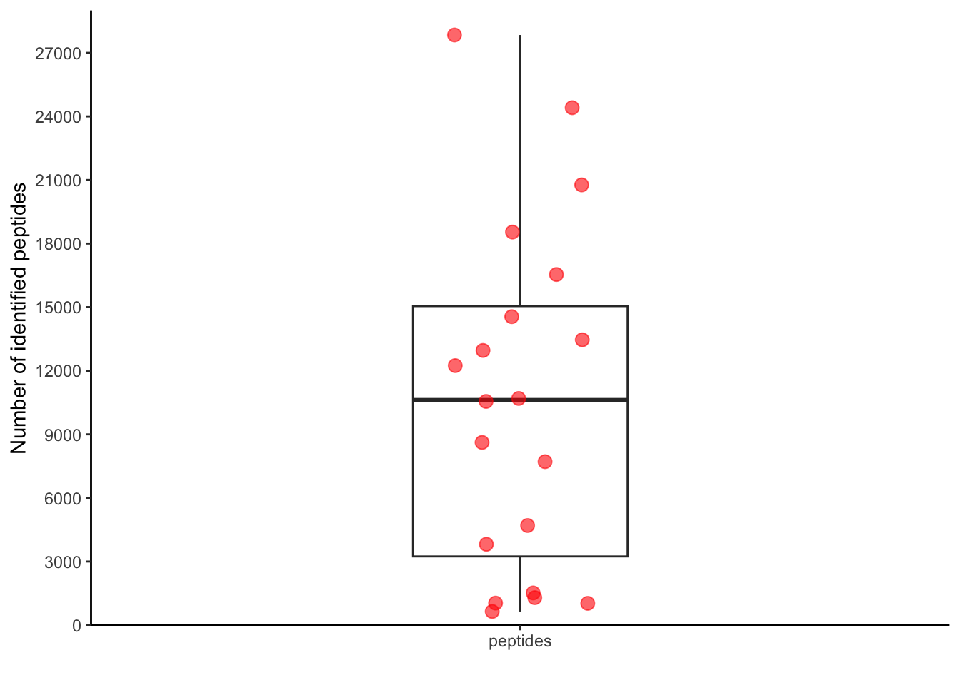

 pivoted_data %>%
  filter(qc=="peptide_identified") %>%
  inner_join(metadata_clean, by="sample") %>%
  ggplot(aes(x=region,
             y=value,
             color=region)) +
  geom_boxplot(width = 0.3,
               outlier.shape = NA, 
               show.legend = FALSE)+ 
  geom_jitter(width= 0.1,
              size=3, 
              show.legend = FALSE,
              alpha = 0.6) +
  scale_y_continuous(expand = c(0,0),
                     limits = c(0, 30000),
                     breaks=seq(0, 30000, by=3000)) +
  labs(x="",
       y="Number of identified peptides") +
  scale_color_manual(values = c("red", "blue")) +
  theme_classic()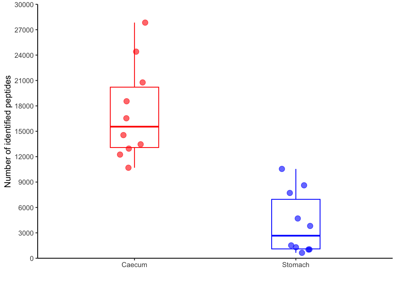

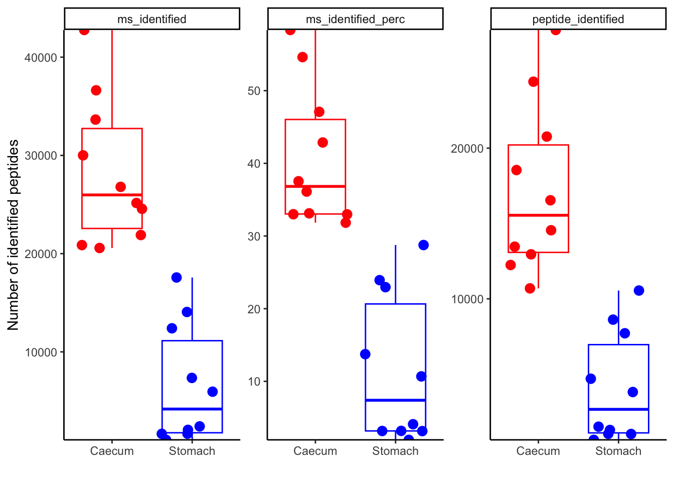
 pivoted_data %>%
   inner_join(metadata_clean, 
              by = "sample"
              ) %>%
   ggplot(aes(x = region,
              y = value,
              color = region
              )
          ) +
   geom_boxplot(outlier.shape = NA, 
                show.legend = FALSE
                ) +
   geom_jitter(size = 3,
               show.legend = FALSE
               ) +
   scale_y_continuous(expand = c(0, 0),
                      # limits = c(0, 27000),
                      # breaks=seq(0, 27000, by=3000)
                      ) +
   labs(x = "",
        y = "Number of identified peptides"
        ) +
   scale_color_manual(values = c("red", "blue")
                      ) +
   theme_classic() +
   facet_wrap(~qc, 
              scales = "free"
              )