Ordination analysis

This tutorial would describe how to perform a Non-metric MultiDimensional Scaling (NMDS) ordination analysis, based on the total protein groups identified in a metaproteomics experiment. NMDS is a distance-based ordination technique, which summarizes the differences or similarities between each pair of sample using any number of response variables. This technique is broadly use in Microbial ecology and metagenomic, metatrascriptomics, metaproteomics and metabolomic analysis. For more details on ordiantion analysis please read Multivariate analyses in microbial ecology and PCoA & NMDS.

For the following analysis we require two data frames 1) metadata describing each sample metadata_metapro.txt and 2) the intensity of the different protein groups across the samples final_proteins.tsv. The protein groups data frame was obtained running a set of metaproteomic raw files in the iMetaLab software.

Set up working space and load data

# libraries ----------------------
library(tidyverse)
library(vegan)

# data------------------
df_proteins <- read_tsv("../../project/rawdata/final_proteins.tsv")

metadata <- read.table(file = "../../project/rawdata/metadata_metapro.txt",
                       header = TRUE,
                       sep = "\t",
                       check.names = FALSE)

Cleaning metadata

First we need to clean our metadata. This specific dataframe has some issues that can create noise during the analysis:

Bad variable naming
The variable rawfiles contain dots (.)
The variable Abschnitt contains spaces and correspond to more than one variable.

We can solve this problems: 1) first renaming the variables using the function rename(), 2) then we can replace the dots (.) for underscores using the functions mutate() and str_replace(), and finally 3) we can separate the variable section into two new variables using the function separate().

metadata <- read.table(file = "../../project/rawdata/metadata_metapro.txt",
                       header = TRUE,
                       sep = "\t",
                       check.names = FALSE) %>% 
  rename(rawfile=Probenname, section=Abschnitt) %>% 
  mutate(rawfile = str_replace(rawfile, "\\.", "_")) %>% 
  separate(section,
           into = c("section", "origin"),
           sep = "\\s") 

metadata[1:5,]

  rawfile  section  origin
1     9_1  Stomach Digesta
2     9_3  Stomach  Mucosa
3     9_4  Stomach  Mucosa
4     9_5  Stomach  Mucosa
5     9_6 Duodenum Digesta

Calculate protein relative abundance

rel_abundance_df <- df_proteins %>%
  rename(proteinid = `Protein IDs`) %>% 
  select(proteinid, contains("Intensity"), -Intensity) %>% 
  pivot_longer(-proteinid, names_to = "rawfile", values_to = "intensity") %>%
  mutate(intensity = as.numeric(intensity),
         rawfile = str_remove(rawfile, "Intensity ")) %>% 
  group_by(rawfile) %>% 
  mutate(rel_abundance = 100*(intensity/sum(intensity))) %>%
  select(proteinid, rawfile, rel_abundance) %>% 
  pivot_wider(names_from = rawfile, values_from = rel_abundance)

Transform the Protein groups data frame

# Create a matrix and transpose data--------------
matrix <- rel_abundance_df[2:21] %>% 
  t()

Non-metric MultiDimensional Scaling (NMDS)

#Calculate distance -----------------
nmds1 <- metaMDS(matrix,  #perform nmds
                 distance = "bray", 
                 try = 20, 
                 trymax = 100, 
                 maxit = 1000, 
                 k = 3)

Run 0 stress 0.0393017 
Run 1 stress 0.03930164 
... New best solution
... Procrustes: rmse 0.000159104  max resid 0.0003476246 
... Similar to previous best
Run 2 stress 0.04066654 
Run 3 stress 0.03930173 
... Procrustes: rmse 0.0001697639  max resid 0.0003891454 
... Similar to previous best
Run 4 stress 0.05920848 
Run 5 stress 0.05922803 
Run 6 stress 0.1882621 
Run 7 stress 0.04063187 
Run 8 stress 0.04066681 
Run 9 stress 0.0425669 
Run 10 stress 0.04066647 
Run 11 stress 0.04063228 
Run 12 stress 0.03930165 
... Procrustes: rmse 0.0001042094  max resid 0.00020394 
... Similar to previous best
Run 13 stress 0.04063213 
Run 14 stress 0.04063194 
Run 15 stress 0.04063198 
Run 16 stress 0.03930161 
... New best solution
... Procrustes: rmse 3.433133e-05  max resid 7.765347e-05 
... Similar to previous best
Run 17 stress 0.04063211 
Run 18 stress 0.04063201 
Run 19 stress 0.04066651 
Run 20 stress 0.03980541 
*** Best solution repeated 1 times

Check the ordination analysis

Using some vegan functions we can check the raw plot of our ordination and how good the analysis fot to our data. It is recommended that the stress of the analysis is lower than 0.2

# qc checking
ordiplot(nmds1, display = "sites")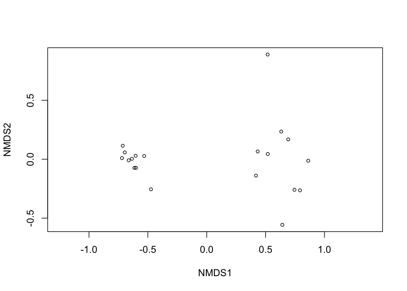

nmds1$stress

[1] 0.03930161

stressplot(nmds1)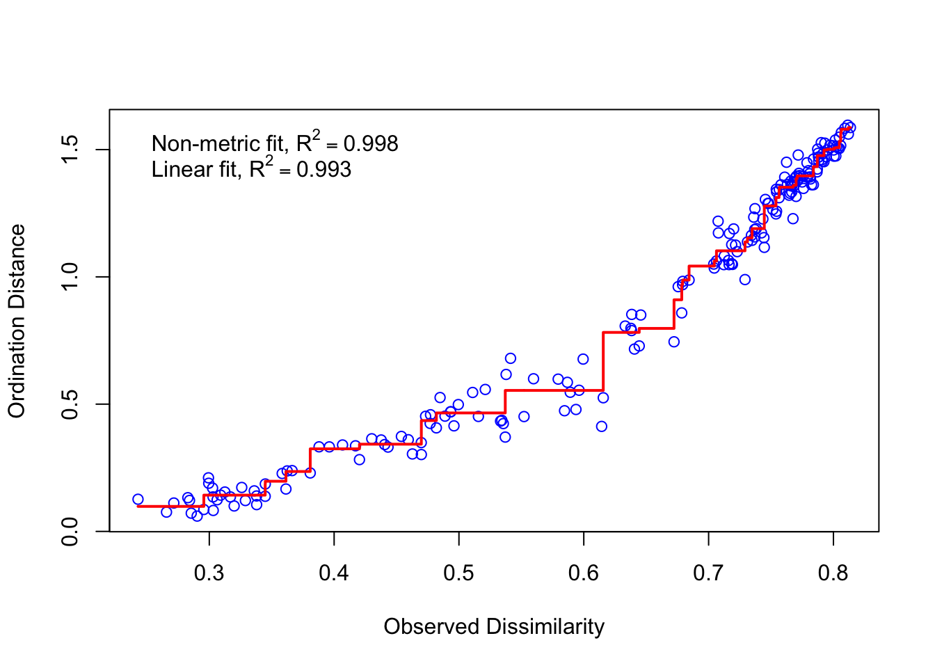

Large scatter around the line suggests that original dissimilarities are not well preserved in the reduced number of dimensions. Looks pretty good in this case

Extract the NDMS scores

We need to extract the scores from the NMDS and combined them with the metadata. In this way we can label each of our samples based on their metadata.

#Extracting scores
data_scores <- as.data.frame(scores(nmds1, display=c("sites")))

#Addd metadata to dataframe
data_scores$rawfile <- as.character(row.names(data_scores)) 

#joing metadata with nmds scorres
data_nmds <- left_join(data_scores, metadata, by = "rawfile")

data_nmds$section <- factor(data_nmds$section,
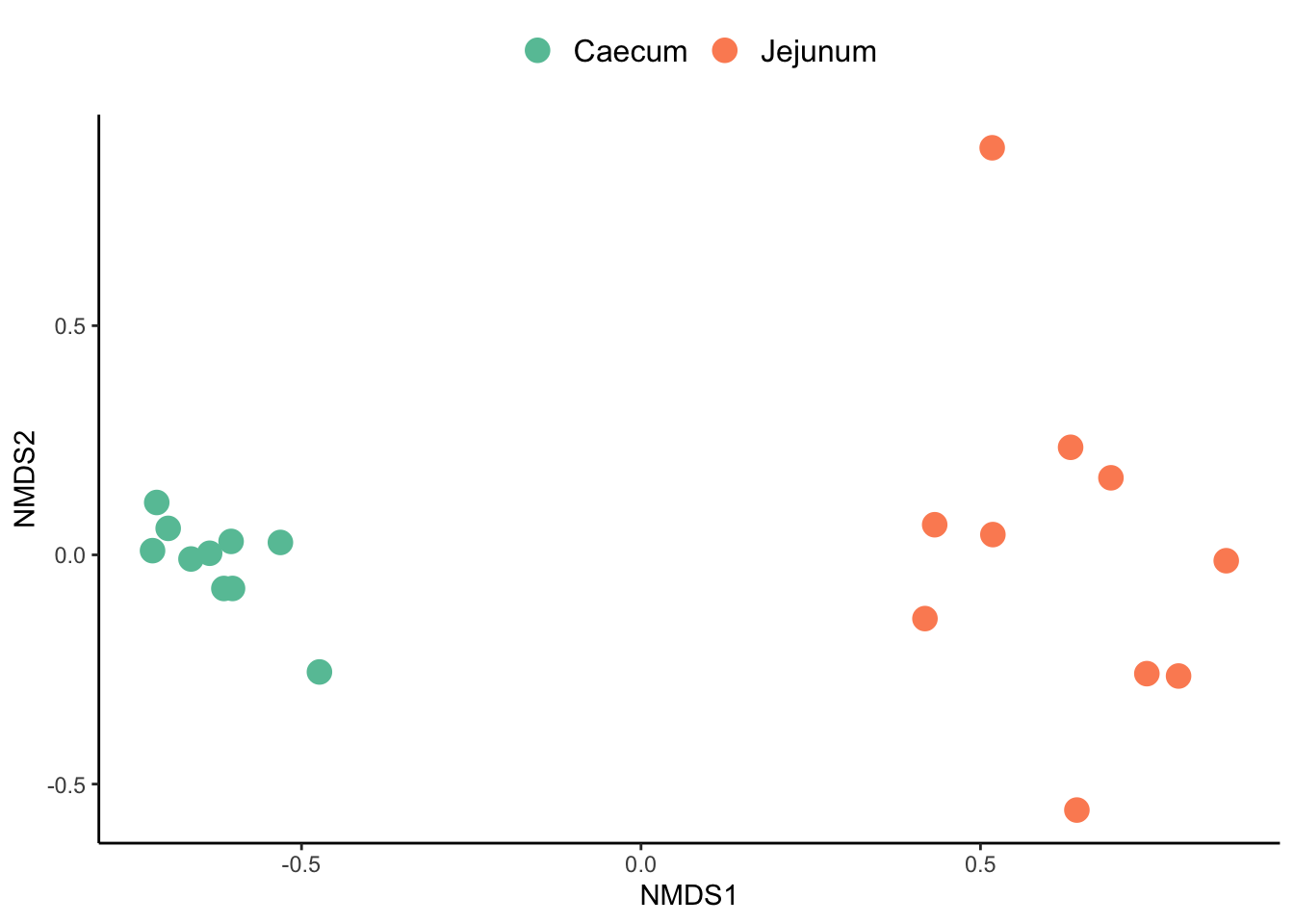
                             levels = c("Caecum", "Jejunum"))#Extracting scores

Create a plot with ggplot

data_nmds %>%
  ggplot() +
  geom_point(aes(x = NMDS1,
                 y = NMDS2,
                 colour =section),
             size = 4
             #alpha = 0.7
  ) +
  scale_color_manual(values = c('#66C2A5','#FC8D62')) +
  theme_classic() +
  theme(panel.background = element_blank(), #remove background
        panel.grid.major = element_blank(), #remove grid
        panel.grid.minor = element_blank(),#remove grid
        legend.title = element_blank(),
        legend.text = element_text(size=12),
        legend.position = "top") #remove legend title