#This function convert cm values to meters.
cm_to_meters <- function(cm) {
cm / 100
}
cm_to_meters(100)[1] 1A function is a set of arguments or commands organized together to perform a specific task. R has a large number of pre installed in-built functions, however the user can create its own functions or install new ones from available packages. For example, the library Tidyverse is a collection of eight different packages functions.
What are the different parts of a function?
Function Name − This is the actual name of the function. It is stored in R environment as an object.
Arguments − An argument is an option that modify the default behaviour of the function. When a function is invoked, you pass a specific value to the argument. Arguments are optional, that means that functions can be use with no arguments.
Function Body − The function body contains all the code that defines what the function does.
function_name <- function(arg_1, arg_2, …) {
   Function_body
}
Lets write a simple function to convert cm to meters. Affter running the function with the value 100, we get the result in meters.
It is not common for beginers to write functions as we tend to use those pre-build in R or from other packages. However, learning to write function is important as we can solve some specific task.
#This function convert cm values to meters.
cm_to_meters <- function(cm) {
  cm / 100
}

cm_to_meters(100)
[1] 1The following list compile several functions, pre-build or from the Tidyverse package, that I usually use during microbiome data wrangling. Be aware that most of the information about the functions was taken from R-help and documentation. If you want to use the help function, write the question mark symbol before the function name (e. g ?setwd()).
Get or Set Working Directory
setwd() is used to set the working directory for the current R session. The selected directory would be consider the root folder.
Example:
setwd("documents/project")
Install and load libraries
install.packages() Download and install packages from CRAN-like repositories or from local files. This function must be use once if the require package is not installed.
library() Load pre-install packages. This function must be use every time a new session starts
Example:
install.packages("Tidyverse")
library(Tidyverse)
read.table()Reads a file in table format and creates a data frame from it, with cases corresponding to lines and variables to fields in the file.
read_tsv() and read_csv() are special cases of the more general read_delim(). They’re useful for reading the most common types of flat file data, comma separated values and tab separated values, respectively.
Example:
read.table(file = "documents/data.txt", header = TRUE, sep = "\t")
R can also be use as a calculator, it is more powerful than that, as many arithmetic function are pre-built in the software. In this way, you can used arithmetic operators like +, -, *, to perform arithmetic calculations.
| Operator | Operation | Output |
|---|---|---|
| x+y | Addition | 15 |
| x – y | Subtraction | 5 |
| x * y | Multiplication | 50 |
| x / y | Division | 2 |
| x ^ y | Exponent | 10^5 |
| x %% y | Modulus | 0 |
You can also use logical operators to perform boolean operation.
| ! | – | NOT |
|---|---|---|
| & | – | AND (Element wise) |
| && | – | AND |
| | | – | OR (Element wise) |
| || | – | OR |
| ! | – | NOT |
Additional, relational operators can be used to compare two values or variables.
| Greater than | x>y | Output: TRUE |
|---|---|---|
| Less than | x<y | Output: FALSE |
| Greater than and equal to | x>=y | Output: TRUE |
| Less than and equal to | x<=y | Output: FALSE |
| Equal to | x==y | Output: FALSE |
| Not equal to | x!=y | Output: TRUE |
However, R also has more complex pre-build function that you can use to transform or create variable, Some of the most common function are:
mean() generic function for the (trimmed) arithmetic mean.
sum() returns the sum of all the values present in its arguments.
sd() this function computes the standard deviation of the values in x. If na.rm is TRUE then missing values are removed before computation proceeds.
max(), min() returns the (regular or parallel) maxima and minima of the input values.
ggplot2 is a system for creating graphics, based on The Grammar of Graphics. You provide the data as a dataframe, tell ggplot2 how to map variables to aesthetics, what graphical geometries to use, and it takes care of the details.
ggplot() initializes a ggplot object. It can be used to declare the input data frame for a graphic and to specify the set of plot aesthetics intended to be common throughout all subsequent layers unless specifically overridden.
geom functions
There are different functions to represent geometric figures or more specifically types of graphs. The most common type of figures are: geom_bar(), geom_boxplot(), geom_line(), geom_point(). You can check all types here ggplot2
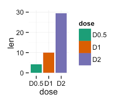
Lets take barplots as examples. There are two types of bar charts: geom_bar() and geom_col(). geom_bar() makes the height of the bar proportional to the number of cases in each group (or if the weight aesthetic is supplied, the sum of the weights). If you want the heights of the bars to represent values in the data, use geom_col() instead.
Scale functions
There are different functions to represent the scales of the data in the plots using R. Those functions can be applied to the x or y axis. The most common type of scales are: scale_x_continuous(), scale_y_continuous(), scale_x_discrete(), scale_y_discrete(), scale_x_log10(), scale_y_log10().
The function scale_y_continuous() can be use to format the y-axis of a continuous variable. For example you can introduce breaks and limits.
labs() Modify axis, legend, and plot labels. Good labels are critical for making your plots accessible to a wider audience. Always ensure the axis and legend labels display the full variable name. Use the plot title and subtitle to explain the main findings. It’s common to use the caption to provide information about the data source. tag can be used for adding identification tags to differentiate between multiple plots.
Themes
theme() is a powerful way to customize the non-data components of your plots: i.e. titles, labels, fonts, background, gridlines, and legends. Themes can be used to give plots a consistent customized look. ggplot has several pre-build themes like: theme_classic() and theme_minimal()
Example:
ggplot(data = data_clean) +
  geom_boxplot(x = groups,
               y = abundance) +
  scale_y_continuous(limits = c(0, 0),
                     breaks = seq(0, 100, 10)) +
  labs(y = "Relative abundance (%)",
       x = "Treatment") +
theme_classic()rename() changes the names of individual variables using new_name = old_name syntax.
separate() can separate a character column into multiple columns with a regular expression or numeric locations.
select() select (and optionally rename) variables in a data frame, using a concise mini-language that makes it easy to refer to variables based on their name (e.g. a:f selects all columns from a on the left to f on the right). You can also use predicate functions like is.numeric to select variables based on their properties.
Data frames can be joined based on different vareiables that they shared. The mutating joins add columns from y to x, matching rows based on the keys:
inner_join(): includes all rows in x and y.
left_join(): includes all rows in x.
right_join(): includes all rows in y.
full_join(): includes all rows in x or y.
If a row in x matches multiple rows in y, all the rows in y will be returned once for each matching row in x.
filter() function is used to subset a data frame, retaining all rows that satisfy your conditions. To be retained, the row must produce a value of TRUE for all conditions. Note that when a condition evaluates to NA the row will be dropped. Conditions acan be stablish using the logical and relational operators.
pivot_longer() “lengthens” data, increasing the number of rows and decreasing the number of columns. The inverse transformation is pivot_wider()
group_by() takes an existing data frame and converts it into a grouped data frame where operations are performed “by group”. ungroup() removes grouping. group_by() is usually cvombined with summarize() and mutate().
summarize() creates a new data frame. It will have one (or more) rows for each combination of grouping variables; if there are no grouping variables, the output will have a single row summarising all observations in the input. It will contain one column for each grouping variable and one column for each of the summary statistics that you have specified.
mutate() adds new variables and preserves existing ones; transmute() adds new variables and drops existing ones. New variables overwrite existing variables of the same name. Variables can be removed by setting their value to NULL.